Adaptive Radix Tree
Exploring & Explaining a Fast Sorted Map

This and the following chapters are from a forthcoming book: Adaptive Radix Tree: Sorted Maps For Fun & Profit
Chapter 0 — What’s a trie?
This tutorial assumes you’re a Go programmer who’s used map[K]V and has reached for a sorted map at some point — google/btree, google/btree, or one of the third-party red-black tree libraries — and got a feel for the API. It does not assume you know what a trie is or how an Adaptive Radix Tree differs from one.
Each chapter builds a working sorted map. Chapter 1 is the simplest imaginable trie. Chapters 2 through 7 each add one decision: lazy expansion, path compression, smaller node types, polymorphism. By chapter 8 you can read the project’s main art.Tree source as a known artifact rather than a wall of code. This chapter is just the primer — no Go yet.
The premise
A sorted map is a map[K]V whose iteration order is the natural ascending order of K, not insertion order or hash order. The operations are familiar:
Put(k, v) // insert or replace
Get(k)    // (v, ok)
Delete(k) // remove if present
Len()     // count
Range(kFrom, kTo)     // iterator in ascending key order
Two well-known data structures offer this API:
Hash maps with side indexes (e.g.
map[K]Vplus a sorted slice you maintain by hand). Lookups are O(1), but every mutation costs O(n) on the slice or O(log n) on a heap, and the iteration order is whatever you paid to maintain.Self-balancing BSTs — red-black, AVL, B-tree. Lookups, inserts, and deletes are O(log n); iteration is a tree walk. These compare keys as opaque blobs: every comparison reads every byte of the key until it finds a difference.
Tries take the third path: don’t compare keys; walk them.
The trie idea
A trie (”retrieval tree”, traditionally pronounced try) is a tree where each edge is labelled with one element of the key (a byte, in our case), and the path from root to a node is the prefix of every key reachable below it. There is no key comparison. Lookup reads the key byte-by-byte and follows the edge labelled with that byte.
The trie was invented during the Cambrian data structure explosion.
René de la Briandais (1959) — “File Searching Using Variable Length Keys,” Proceedings of the Western Joint Computer Conference. First published description of the structure.
Edward Fredkin (1960) — “Trie Memory,” Communications of the ACM 3(9):490–499. Coined the name trie (pronounced “try”) from the middle syllable of retrieval.
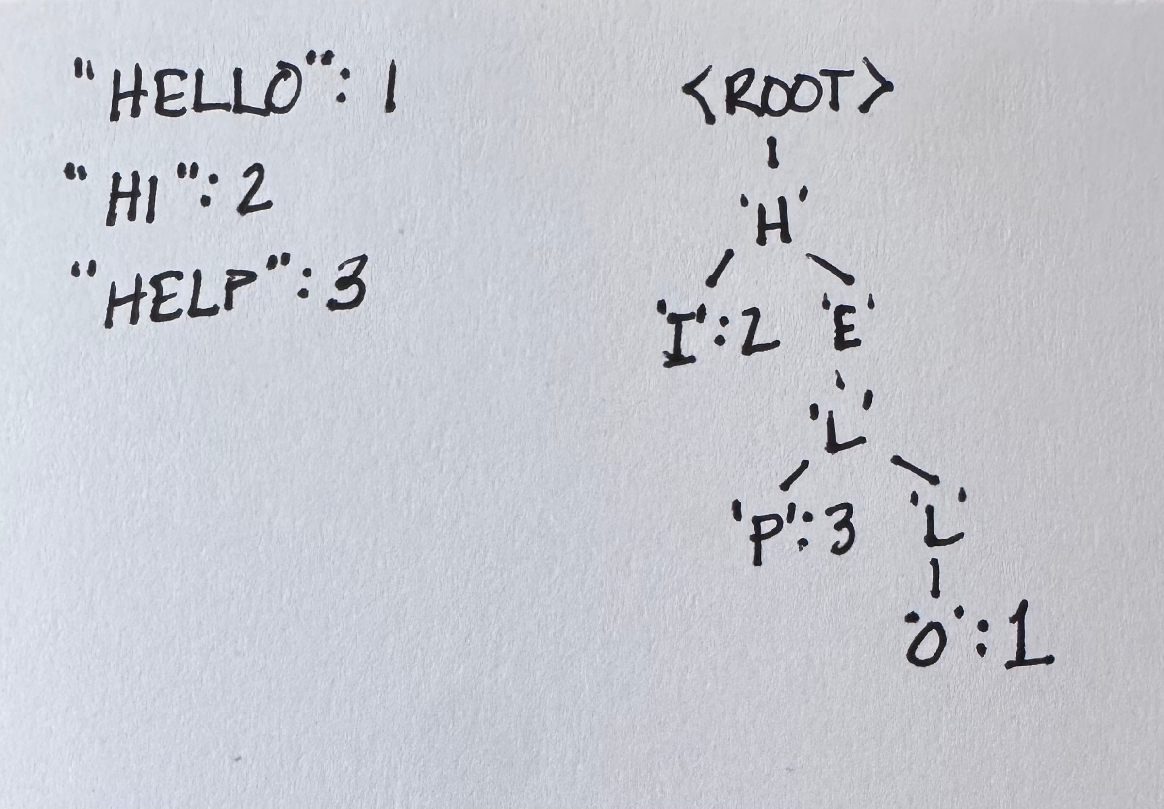
An ASCII picture of the keys {hello:1, hi:2, help:3}:
Two consequences fall out for free:
Sorted iteration is automatic. At each node, visit children in ascending byte order. The yielded keys appear in byte-wise sorted order with no comparisons and no balancing.
Shared work for shared prefixes. A lookup of
helpand a lookup ofhellotraverse the same first four edges. The per-byte cost depends on the keys’ shape, not on the size of the map.
What a trie costs
The honest tradeoffs are equally direct:
One node-traversal per byte. A 16-byte key is 16 pointer dereferences down the tree. If the tree is bigger than your L1 cache, that’s 16 cache misses. A B-tree comparing the same key against a few interior keys is fewer dereferences but each comparison reads more bytes; the right answer depends on the workload.
Wasted nodes for sparse keysets. Every byte position where any key has a unique value gets its own node. If your keys are random 16-byte blobs, almost every level branches, and you pay for one inner node per byte per key. Chapter 1 makes this visible: ~33 MB to store 1 000 random 16-byte keys in the simplest possible trie.
The book is structured according to the principles of David Parnas and Paul Clements's 1986 paper A Rational Design Process: How and Why to Fake It. The first chapter introduces a simple-but-slow implementation. Each of the seven succeeding chapters addresses the slowness of the previous chapter until we have the whole ART.
Only full-sized nodes (chapter 1)—we build a whole working tree out of nodes that assume all 256 children are valid. (Foreshadowing—this will turn out to be a useful disaster.)
Lazy expansion (chapter 2)—stop allocating inner nodes along a tail with no siblings.
Path compression (chapter 3)—let one node represent several consecutive bytes when none of them branch.
Small node type (chapter 4)—stores up to 4 keys.
Polymorphism (chapter 5)—we’re going to add more node sizes, so why don’t we make it easy? (Make the hard change easy, then make the easy change.)
In between node types (chapters 6 & 7)—save space at the cost of computation by filling in nodes with up to 16 & then 48 keys. (Of course it’s more interesting than a simple tradeoff when space saving reduces memory pressure & thus saves time.)
Polish (chapter 8)—inline-key buffers, embedded headers, a reused path buffer for
Range. Allocations per key drop to roughly one.
By chapter 8 the implementation is the same shape as the production art.Tree in the parent package. You will have built it, decision by decision, and you will have measured what each decision was worth.
Viktor Leis, Alfons Kemper, and Thomas Neumann at the Technical University of Munich published the adaptive radix tree first.
Published as “The Adaptive Radix Tree: ARTful Indexing for Main-Memory Databases” at ICDE 2013. PDF: https://db.in.tum.de/~leis/papers/ART.pdf
Onward to chapter 1, where we build the disaster. Well, the naive, memory wasteful version.